mujoco-200-tutorials-Lec7: Linear Quadratic Regulator for Under-actuated Double Pendulum
Balance control of acrobot!
underactuated 2 link open chain에서 첫번째 joint에 actuator가 있다면 pendubot, 두번째 joint에 actuator가 있다면 acrobot이다. underactuated system은 DOF > # of actuator인 system을 말한다. 이번 경우 DOF=2, # of actuator=1
다음과 같이 출력변수 T를 control하면 된다.
\[T = -Ku = -K_1q_1 -K_2\dot{q_1} -K_3q_2 -K_4\dot{q_2}\]임의로 가중행렬 R,Q를 설정하고, Linear quadratic regulator(LQR)의 제어파라미터인 gain matrix K를 matlab으로 결정할 수 있다. (원래는 liccati differential equation을 풀어야한다.)
Q가 줄어들수록 input최적화효과가 줄어들기때문에 gain matrix K가 커지고, position 제어효과가 좋아질 것이다.
cost function은 다음과 같다.
\[J=\int \limits _{t_{0}}^{t_{1}}\left(x^{T}Qx+u^{T}Ru\right)dt\]따라서 가중행렬 Q,R에 따라 position을 원점으로 유지하며 최소한의 torque를 입력하는 것이 이번 lqr controller의 설계목표이다!
Full code
lqr controller modeling
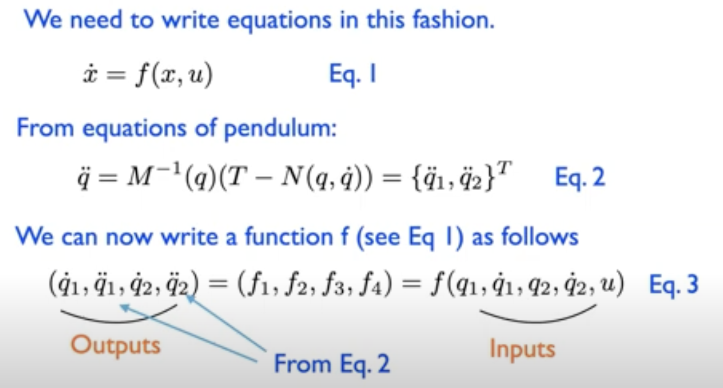
acrobot의 dynamics는 다음과 같다.
\(M(q)\ddot{q}\) + qfrc_biasd \(= T\)
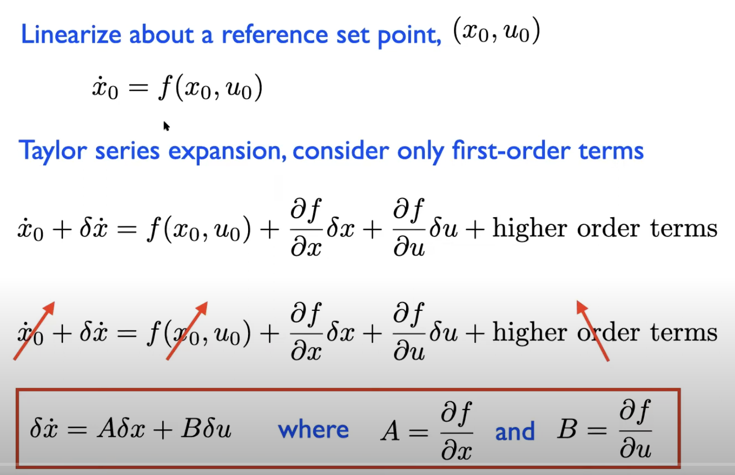
state variable을 \([q_1,\dot{q_1},q_2,\dot{q_2}]\)로 두고, acrobot의 dynamics가 다음과 같은 linear approximation을 만족한다고 가정하고, 시뮬레이션을 통해 \(\dot{\delta x}, \delta x, \delta u\)를 구해서 A, B를 찾아낸다.
state input을 joint에 전달하고, dynamics로부터 도출 및 sensing(d->qvel)을 통해 state output을 출력하는 함수 f를 만든다.
make model f for calculation A,B (not for control callback!)
A,B 계산을 위해 state의 입출력이 필요하므로 그걸 구현하는 함수를 만들어준다.
1
2
3
4
5
6
7
8
9
10
11
12
13
14
15
16
17
18
19
20
21
22
23
24
25
26
27
28
29
30
31
32
33
34
35
36
37
38
39
40
void f(const mjModel* m, mjData* d, double input[5], double output[4]) {
	// state = [q1, q1dot, q2, q2dot]
	// input = [q1, q1dot, q2, q2dot u]
	// output = [q1dot, q1ddot, q2dot, q2ddot]
	d->qpos[0] = input[0];
	d->qvel[0] = input[1];
	d->qpos[1] = input[2];
	d->qvel[1] = input[3];
	d->ctrl[0] = input[4];
	mj_forward(m,d);
	double q1dot, q2dot;
	q1dot = d->qvel[0];
	q2dot = d->qvel[1];
	// dynamics
	// Mqacc + qfrc_bias = ctrl
	const int nv = 2;
	double M[nv*nv] = {0};
	// void mj_fullM(const mjModel* m, mjtNum* dst, const mjtNum* M);
	mj_fullM(m,M,d->qM);
	double det_M = M[0]*M[3] - M[1]*M[2];
	double inv_M[nv*nv] = {M[3],-M[1],-M[2],M[0]};
	for(int i=0; i<4; i++) {
		inv_M[i] /= det_M;
	}
	// f = ctrl - qfrc_bias
	double f[2] = {0};
	f[0] = (0 - d->qfrc_bias[0]); // joint1 is no control
	f[1] = (d->ctrl[0] - d->qfrc_bias[1]);
	// qacc = inv_M(ctrl - qfrc_bias)
	double qacc[2] = {0};
	// void mju_mulMatVec(mjtNum* res, const mjtNum* mat, const mjtNum* vec, int nr, int nc);
	mju_mulMatVec(qacc, inv_M, f, 2, 2);
	double q1ddot, q2ddot;
	q1ddot = qacc[0];
	q2ddot = qacc[1];
	output[0] = q1dot;
	output[1] = q1ddot;
	output[2] = q2dot;
	output[3] = q2ddot;
}
calculation A,B for system using first derivative
descrete system이므로, unit time에 대해 perterbation( \(\delta x, \delta u\) )을 줘서,
f의 x에 대한 derivative A,
f의 u에 대한 derivative B
를 계산한다.
1
2
3
4
5
6
7
8
9
10
11
12
13
14
15
16
17
18
19
20
21
22
23
24
25
26
27
28
29
30
31
32
33
34
35
36
37
38
39
40
41
42
43
44
45
46
47
48
49
50
51
52

void init_controller(const mjModel* m, mjData* d)
{
	double input[5] = {0};
	double output[4] = {0};
	double perturb = 0.001;

	double f0[4] = {0};
	f(m,d,input,output);
	for(int i=0; i<4; i++){
		f0[i] = output[i];
	}

	double A[4][4] = {0};

	for(int j=0; j<4; j++) {
		for(int i=0; i<5; i++){
			input[i] = 0;
		}
		input[j] = perturb;
		f(m,d,input,output);

		for(int i=0; i<4; i++){
			A[i][j] = (output[i]-f0[i])/perturb;
		}
	}
	// printf("A = [...\n");
	// for(int i=0; i<4; i++) {
	// 	for(int j=0; j<4; j++) {
	// 		printf("%f ", A[i][j]);
	// 	}
	// 	printf(";\n");
	// }
	// printf("];\n\n");

	double B[4] = {0};
	for(int i=0; i<5; i++){
		input[i] = 0;
	}
	input[4] = perturb;
	f(m,d,input,output);
	for(int i=0; i<4; i++){
		B[i] = (output[i]-f0[i])/perturb;
	}
	// printf("B = [...\n");
	// for(int i=0; i<4; i++) {
	// 	printf("%f ", B[i]);
	// 	printf(";\n");
	// }
	// printf("];\n\n");
}
calculation lqr by MATLAB
계산된 A,B와 함께 적당한 가중행렬 Q,R을 설정하여 gain matrix K를 계산한다.
1
2
3
4
5
6
7
8
9
10
11
12
13
14
15
16
17
18
19
20
21

A = [...
0.000000 1.000000 0.000000 0.000000 ;
12.592667 0.000000 -12.545599 0.000000 ;
0.000000 0.000000 0.000000 1.000000 ;
-16.758859 0.000000 46.016228 0.000000 ;
];

B = [...
0.000000 ;
-4.266066 ;
0.000000 ;
13.647575 ;
];

rho = 0.001;
Q = eye(4);
R = rho;

K = lqr(A,B,Q,R)
apply optimal input with noise
task space에서 external force와 joint에 가해지는 torque에 noise를 가해도 stable하게 contol가능한지 확인해본다.
1
2
3
4
5
6
7
8
9
10
11
12
13
14
15
16
17
18
19
20
21
22
23
24
void mycontroller(const mjModel* m, mjData* d)
{
	// write control here
	if(lqr)
	{
		double K[4] = {-3.9288,   -1.4486,   -1.0113,   -0.4192};
		d->ctrl[0] = -K[0]*1000*d->qpos[0]-K[1]*1000*d->qvel[0]-K[2]*1000*d->qpos[1]-K[3]*1000*d->qvel[1];

		double noise;
		// mjtNum mju_standardNormal(mjtNum* num2);
		mju_standardNormal(&noise);
		int body = 2;
		d->xfrc_applied[6*body+0]=10*noise;
		d->qfrc_applied[0] = noise;
		d->qfrc_applied[1] = noise;
	}

  //write data here (dont change/dete this function call; instead write what you need to save in save_data)
  if ( loop_index%data_chk_period==0)
    {
      save_data(m,d);
    }
  loop_index = loop_index + 1;
}